Is This Bayesian? You Know Im a Strict Bayesian
Getting Started
Bayesian Statistics
Hard to believe at that place was once a controversy over probabilistic statistics

This article builds on my previous article about Bootstrap Resampling.
Introduction to Bayes Models
Bayesian models are a rich class of models, which can provide attractive alternatives to Frequentist models. Arguably the most well-known feature of Bayesian statistics is Bayes theorem, more than on this afterwards. With the recent advent of greater computational ability and general credence, Bayes methods are now widely used in areas ranging from medical inquiry to natural language processing (NLP) to understanding to spider web searches.
In the early 20th century in that location was a large debate about the legitimacy of what is at present chosen Bayesian, which is substantially a probabilistic manner of doing some statistics — in contrast to the "Frequentist" military camp that we are all intimately familiar with. To utilize the parlance of our times, it was the #Team Jacob vs #Team Edward debate of its fourth dimension, among statisticians. The argument is now moot equally most everyone is both Bayesian and Frequentist. A adept heuristic is that some problems are better handled by Frequentist methods and some with Bayesian methods.
By the end of this article I hope you lot can appreciate this joke: A Bayesian is one who, vaguely expecting a horse, and catching a glimpse of a donkey, strongly believes she has seen a mule!
History
A limited version of Bayes theorem was proposed past the eponymous Reverend Thomas Bayes (1702–1761). Bayes' interest was in probabilities of gambling games. He as well was an avid supporter of Sir Isaac Newton'southward newfangled theory of calculus with his amazingly entitled publication, "An Introduction to the Doctrine of Fluxions, and a Defence of the Mathematicians Against the Objections of the Author of The Analyst."
In 1814, Pierre-Simon Laplace published a version of Bayes theorem similar to its modern class in the "Essai philosophique sur les probabilités." Laplace applied Bayesian methods to problems in angelic mechanics. Solving these problems had great applied implications for ships in the late 18th/early on 19th centuries. The geophysicist and mathematician Harold Jeffreys extensively used Bayes' methods.
WWII saw many successful applications of Bayesian methods:
- Andrey Kolmagorov, a Russian (née Soviet) statistician used Bayes methods to profoundly improve artillery accurateness
- Alan Turing used Bayesian models to suspension High german U-boat codes
- Bernard Koopman, French born American mathematician, helped the Allies ability to locate German language U-boats by intercepting directional radio transmissions
The latter one-half of the 20th century lead to the following notable advances in computational Bayesian methods:
- Statistical sampling using Monte Carlo methods; Stanislaw Ulam, John von Neuman; 1946, 1947
- MCMC, or Markoff chain Monte Carlo; Metropolis et al. (1953) Journal of Chemical Physics
- Hastings (1970), Monte Carlo sampling methods using Markov chains and their awarding
- Geman and Geman (1984) Stochastic relaxation, Gibbs distributions and the Bayesian restoration of images
- Duane, Kennedy, Pendleton, and Roweth (1987), Hamiltonian MCMC
- Gelfand and Smith (1990), Sampling-based approaches to calculating marginal densities.
Bayesian vs Frequentist views
With greater computational power and general acceptance, Bayes methods are now widely used in areas ranging from medical research to natural language understanding to web search. Amid pragmatists, the common belief today is that some problems are better handled by frequentist methods and some with Bayesian methods.
From my start article on the Central Limit Theorem (CLT), I established that y'all need "enough data" for the CLT to apply. Bootstrap sampling is a convenient way of obtaining more than distributions that approach your underlying distribution. These are Frequentist tools; but what happens if you have likewise niggling data to reliably utilise the CLT? Every bit a probabilistic Bayesian statistician, I already have some estimates, admittedly, with a niggling bit of guesswork, but in that location is a style of combining that guesswork in an intelligent fashion with my data. And that is what Bayesian statistics is basically all almost — you combine information technology and basically, that combination is a simple multiplication of the two probable probability distributions, the 1 that yous guessed at, and the other one, that for which you have evidence.
The more data y'all accept, the prior distribution becomes less and less of import and Frequentist methods tin be used. Just, with less data, Bayesian's volition requite you lot a meliorate respond.
So how and so practice Bayesian and Frequentist methodologies differ? Simply stated:
- Bayesian methodologies use prior distributions to quantify what is known about the parameters
- Frequentists do not quantify annihilation about the parameters; instead using p-values and confidence intervals (CI'southward) to express the unknowns almost parameters
Both methods are useful, converging with more and more data — but assorted:
Strict Frequentist approach
- Goal is a point gauge and CI
- Outset from observations
- Re-compute model given new observations
- Examples: Mean guess, t-test, ANOVA
Bayesian approach
- Goal is posterior distribution
- Commencement from prior distribution (the guesswork)
- Update posterior (the belief/hypothesis) given new observations
- Examples: posterior distribution of mean, highest density interval (HDI) overlap
Today no i is a strict Frequentist. Bayesian methodologies simply piece of work, that is fact.
Bayes theorem
Bayes theorem describes the probability of an event, based on prior cognition (our guesswork) of conditions that might be related to the upshot, our data. Bayes theorem tells us how to combine these ii probabilities. For example, if developing a illness like Alzheimer's is related to age, then, using Bayes' theorem, a person's age can be used to more reliably appraise the probability that they have Alzheimer's, or cancer, or whatsoever other age-related disease.
Bayes theorem is used to update the probability for a hypothesis; the hypothesis is this guesswork, this prior distribution thing. Prior ways your prior belief, the belief that y'all have earlier y'all take evidence, and information technology is a way to update it. Because you go more than information, y'all update your hypothesis, and so on and then forth.
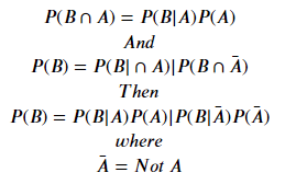
For those who practise non know, or who accept forgotten, let united states derive Bayes theorem from the rule for provisional probability:
Translates to "the probability of A happening given B is the case."
"The probability of B happening given A happens."
Eliminating 𝑃(𝐴∩𝐵) and doing very minor algebra:
or, rearranging terms
Which is Bayes theorem! This describes how 1 finds the conditional probability of effect A given event B.
Applications
You have a disease test, and the probability that you will go a positive examination result given that you take the disease is actually, really high; in other words the test has a very high accuracy rate. The trouble is that there is a probability that you lot will get a positive test result even if yous exercise non have the disease. And that you can but summate from Bayes law. The large indicate is, is that these probabilities are non the same as the probability that you volition get a positive result given the disease is non the same as the probability that yous will have the affliction given a positive result.
These are two different probability distributions. And what makes them so different is the probability of disease and the probability of a positive test result. So if the disease is rare, the probability of disease will be very, very minor.
Disease testing: A = Accept disease, B = Tested positive.
Example
Using Bayes theorem we have deduced that a positive test result for this disease indicates that but ten% of the time the person will actually take the disease, because the incidence rate of the disease is an order of magnitude lower than the false positive rate.
Python example: probabilities of hair and heart colour
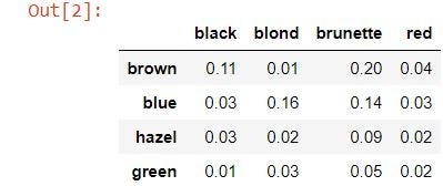
A sample population has the post-obit probabilities of hair and eye color combinations. I will run the code below in a Jupyter Notebook to find the conditional probabilities:
# begin with the imports
import pandas as pd
import numpy as np
import matplotlib
from matplotlib import pyplot as plt
import scipy
import seaborn as sns
import itertools %matplotlib inline # create the dataframe
hair_eye = pd.DataFrame({
'blackness': [0.xi, 0.03, 0.03, 0.01],
'blond': [0.01, 0.sixteen, 0.02, 0.03],
'brunette': [0.two, 0.14, 0.09, 0.05],
'scarlet': [0.04, 0.03, 0.02, 0.02],}, alphabetize=['brown', 'bluish', 'hazel', 'green'])
hair_eye
Northward.B: this is string alphabetize for eye colour rather than a numeric null-based index.
hair_eye.loc['hazel', 'ruby-red'] 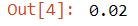
The figures in the tabular array above are the provisional probabilities. Note that in this case:
𝑃(hair|eye)=𝑃(eye|hair)P(hair|eye)=P(center|hair)
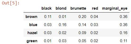
Given these conditional probabilities, it is easy to compute the marginal probabilities by summing the probabilities in the rows and columns. The marginal probability is the probability along one variable (one margin) of the distribution. The marginal distributions must sum to unity (1).
          ## Compute the marginal distribution of each center color
hair_eye['marginal_eye'] = hair_eye.sum(centrality=1)          hair_eye
hair_eye.sum(axis=0) 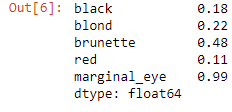
          hair_eye.loc['marginal_hair'] = hair_eye.sum(axis=0)
hair_eye.describe 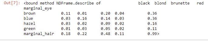
I have blue optics. I wonder what the marginal probabilities of hair color are given that they have blue eyes?
          # probability of bluish eyes given whatever hair color divided past total probability of blueish eyes          # marginal probabilities of pilus color given blue eyes
#blue_black(.03/.36) + blue_brunette(.14/.36) + blue_red(.03/.36) + blue_blond(.16/.36)
blue = hair_eye.loc['blue',:]/hair_eye.loc['blue','marginal_eye']
bluish

Applying Bayes theorem
There is a formulation of Bayes theorem that is user-friendly to use for computational bug considering we do not want to sum all of the possibilities to compute P(B), like in the example higher up.
Here are more facts and relationships most provisional probabilities, largely arising from the fact that P(B) is so difficult to calculate:
Rewriting Bayes theorem:
This is a mess, simply nosotros practise not always demand the complicated denominator, which is the probability of B. P(B) is our actual bear witness, which is hard to come by. Remember that this is probabilistic and that we are working with smaller data samples than nosotros are commonly used to.
Rewriting nosotros get:
Ignoring the constant 𝑘, because it is given that the testify - P(B) - is presumed to be abiding, nosotros get:
Applying the reduced relationship Bayes theorem
We interpret the reduced human relationship higher up as follows:
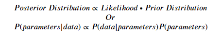
The proportional relationships apply to the observed data distributions, or to parameters in a model (partial slopes, intercept, mistake distributions, lasso constant, e.g.,). The to a higher place equations tell you how to combine your prior conventionalities if you want to call that, which I phone call the prior distribution with your bear witness.
An important dash is that while we cannot speak about exact values we can talk almost distributions; nosotros can talk about the shapes of the curves of the probability distribution curves. What nosotros desire is the and then-chosen posterior distribution. That is what we want. What we exercise is gauge at the prior distribution: what is the probability of A? What is the probability that something is truthful given the data that I accept? What is the probability of A given B? what is the probability that something is true given the data I have? Some people volition rephrase this as what is the probability that my hypothesis A is true given the data B?
I might have very fiddling data. Too lilliputian to practice any Frequentist approaches; merely I tin estimate that with the fiddling small corporeality of information I have, called the likelihood, I tin can estimate the probability that this data would be correct, given my hypothesis that I can calculate directly. Because I have the information, not a lot of data, it is also fiddling for me to actually believe, just I have some data. And I have my hypothesis. And then I can do my calculations on my distributions.
The prior distribution is the probability of my hypothesis, which I do not know — but I can guess it. If I am actually bad at guessing, I am going to say that this prior distribution is a uniform distribution, it could be a Gaussian or whatever other shape. Now if I guess a compatible distribution I am still doing probabilistic statistics, Bayesian statistics, just I am getting actually, really close to what Frequentists would do.
In Bayesian, I will update this prior distribution as I get more information because I volition say, "Hey!" at first I thought it was compatible. Now I run across that this thing, this probability distribution really has a mean somewhere in the middle. And so I am now going to choose a unlike distribution. Or I'one thousand going to modify my distribution to accommodate what I am seeing in my posterior. I am trying to brand this prior distribution look similar in shape to my posterior distribution. And when I say similar in shape, that is really very misleading. What I am trying to do is find a mathematical formula that will mix the probability of A and the probability of A given B similarly. Similar in type that the math, that the equation looks like, as in the formulaic of the question and non the actual probabilities; we call that getting the conjugate prior. This is when y'all search for a distribution that is mathematically similar to what you believe to exist the final distribution. This is formally referred to as searching for a conjugate prior. A beta distribution, because of its flexibility is often, but not e'er, used as the prior.
To reiterate, the hypothesis is formalized equally parameters in the model, P(A), and the likelihood, P(B|A), is the probability of the data given those parameters — this is easy to do, t-tests can do this!
Creating Bayes models
Given prior assumptions about the behavior of the parameters (the prior), produce a model which tells us the probability of observing our information, to compute new probability of our parameters. Thus the steps for working with a Bayes model are:
- Identify data relevant to the inquiry question: e.g., measurement scales of the information
- Ascertain a descriptive model for the data. For instance, option a linear model formula or a beta distribution of (2,ane)
- Specify a prior distribution of the parameters — this the formalization of the hypothesis. For example, thinking the error in the linear model is normally distributed as 𝑁(𝜃,𝜎²)
- Choose the Bayesian inference formula to compute posterior parameter probabilities
- Update Bayes model if more than data is observed. This is key! The posterior distribution naturally updates every bit more data is added
- Simulate information values from realizations of the posterior distribution of the parameters
Choosing a prior
The choice of the prior distribution is very of import to Bayesian analysis. A prior should exist convincing to a skeptical audience. Some heuristics to consider are:
- Domain knowledge (SME)
- Prior observations
- If poor cognition use less informative prior
- Caution: the uniform prior is informative, you need to set the limits on the range of values
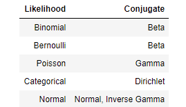
I analytically and computationally simple choice is the before mentioned conjugate prior. When a likelihood is multiplied by a cohabit prior the distribution of the posterior is the aforementioned as the likelihood. Well-nigh named distributions accept conjugates:
Python Example: COVID-19 random sampling
As a wellness official for your metropolis, y'all are interested in analyzing COVID-19 infection rates. Yous make up one's mind to sample 10 people at an intersection while the low-cal is carmine and determine if they test positive for Covid — the test is fast and to avert sampling bias we take the exam to them. The data are binomially distributed; a person tests positive or tests negative — for the sake of simplicity, assume the exam is 100% authentic.
In this notebook case:
- Select a prior for the parameter 𝑝, the probability of having COVID-xix.
- Using data, compute the likelihood.
- Compute the posterior and posterior distributions.
- Try another prior distribution.
- Add more data to our data gear up to updated the posterior distribution.
The likelihood of the data and the posterior distribution are binomially distributed. The binomial distribution has one parameter we need to estimate, 𝑝, the probability. We can write this formally for 𝑘 successes in 𝑁 trials:
The following code computes some basic summary statistics:
          sampled = ['yes','no','yes','no','no','aye','no','no','no','yeah']
positive = [1 if x is 'yeah' else 0 for ten in sampled]
positive 
          North = len(positive) # sample size
n_positive = sum(positive) # number of positive drivers
n_not = Due north — n_positive # number negative
print('Tested positive= %d Tested negative= %d'
            '\nProbability of having COVID-19= %.1f'
% (n_positive, n_not, n_positive / (n_positive+ n_not))) 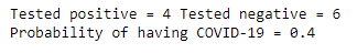
For the prior I will start with a uniform distribution as I exercise not know what to wait re Covid rates:
N = 100
p = np.linspace(.01, .99, num=Northward)
pp = [i./Northward] * North
plt.plot(p, pp, linewidth=2, colour='blue')
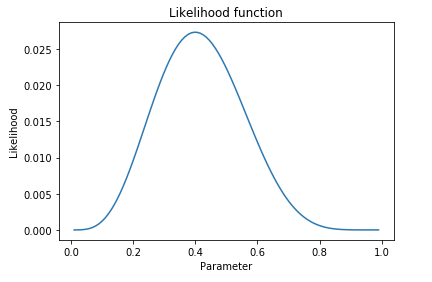
plt.show() Next step: compute the likelihood. The likelihood is the probability of the data given the parameter, 𝑃(𝑋|𝑝). Each observation of each examination as "positive" or "not" is a Bernoulli trial, then I choose the binomial distribution.
          def likelihood(p, data):
            k = sum(data)
            N = len(data)
            # Compute Binomial likelihood
            l = scipy.special.rummage(N, thou) * p**thou * (1-p)**(Due north-k)
            # Normalize the likelihood to sum to unity
            return 50/sum(fifty)          l = likelihood(p, positive)
plt.plot(p, fifty)
plt.title('Likelihood function')
plt.xlabel('Parameter')
plt.ylabel('Likelihood')
plt.show()
Now that we have a prior and a likelihood we can compute the posterior distribution of the parameter 𝑝: 𝑃(𝑝|𝑋).
Due north.B. The computational methods used here are simplified for the purpose of illustration. Computationally efficient lawmaking must be used!
def posterior(prior, like):
post = prior * like # compute the production of the probabilities
return post / sum(mail) # normalize the distribution def plot_post(prior, similar, post, x):
maxy = max(max(prior), max(like), max(post))
plt.figure(figsize=(12, four))
plt.plot(x, like, label='likelihood', linewidth=12, color='black', alpha=.two)
plt.plot(x, prior, label='prior')
plt.plot(x, mail, label='posterior', color='greenish')
plt.ylim(0, maxy)
plt.xlim(0, 1)
plt.title('Density of prior, likelihood and posterior')
plt.xlabel('Parameter value')
plt.ylabel('Density')
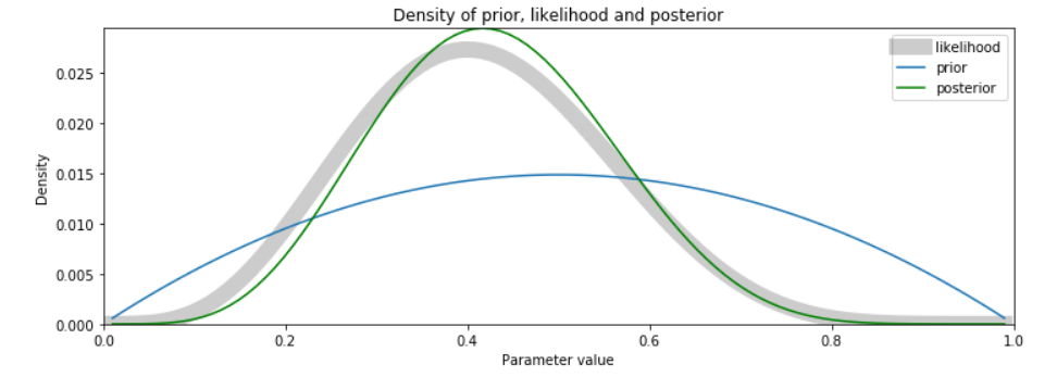
plt.legend()post = posterior(pp, l)
plot_post(pp, fifty, post, p)
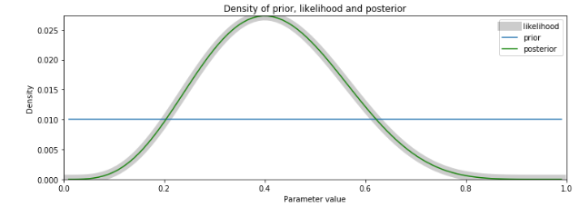
          impress('Maximum of the prior density = %.3f' % max(pp))
print('Maximum likelihood = %.3f' % max(l))
print('MAP = %.3f' % max(post)) 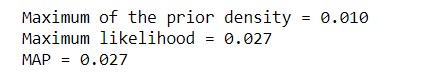
With a compatible prior distribution, the posterior is only the likelihood. The key point is that the Frequentist probabilities are identical to the Bayesian posterior distribution given a compatible prior.
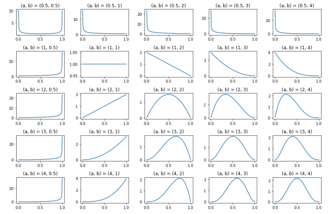
Trying a dissimilar prior
From the chart above, I chose the cohabit prior of the Binomial distribution which is the beta distribution. The beta distribution is divers on the interval 0 ≤ Beta(P|A, B)≤x ≤ Beta(P|A, B)≤ 1. The beta distribution has 2 parameters, 𝑎 and 𝑏, which decide the shape.
          plt.figure(figsize=(12, 8))          alpha = [.v, one, 2, 3, 4]
beta = alpha[:]
x = np.linspace(.001, .999, num=100) #100 samples          for i, (a, b) in enumerate(itertools.production(alpha, beta)):
            plt.subplot(len(alpha), len(beta), i+1)
            plt.plot(x, scipy.stats.beta.pdf(ten, a, b))
            plt.title('(a, b) = ({}, {})'.format(a,b))
plt.tight_layout()
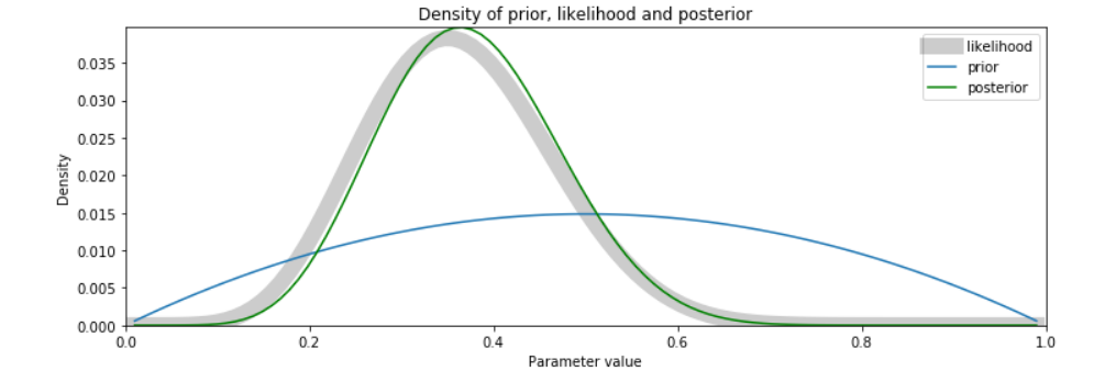
I nevertheless do not know a lot about the behavior of drivers at this intersection who may or may not have COVID-xix, so I pick a rather uninformative or broad beta distribution as the prior for the hypothesis. I cull a symmetric prior with a=ii and b=ii:
          def beta_prior(x, a, b):
            fifty = scipy.stats.beta.pdf(p, a, b) # compute likelihood
            return l / l.sum() # normalize and return          pp = beta_prior(p, ii, ii)
mail = posterior(pp, l)
plot_post(pp, l, mail, p)
Accept note that the fashion of the posterior is close to the way of the likelihood, only has shifted toward the mode of the prior. This behavior of Bayesian posteriors to be shifted toward the prior is known as the shrinkage belongings: the tendency of the maximum likelihood point of the posterior is said to shrink toward the maximum likelihood point of the prior.
Updating the Bayesian model
Let u.s.a. update the model with ten new observations to our data gear up. Note that the more observations added to the model moves the posterior distribution closer to the likelihood.
N.B. With big datasets, it might require HUGE amounts of information to encounter convergence in behavior of the posterior and the likelihood.
          new_samples = ['yes','no','no','no','no',
            'yep','no','yes','no','no'] # new information to update model, due north = 20
new_positive = [1 if x is 'aye' else 0 for ten in new_samples]          50 = likelihood(p, positive+ new_positive)
post = posterior(pp, 50)
plot_post(pp, l, post, p)
Credible Intervals
A credible interval is an interval on the Bayesian posterior distribution. The credible interval is sometimes called the highest density interval (HDI). For instance, the 90% credible interval encompasses xc% of the posterior distribution with the highest probability density. Information technology can exist confusing since both credible intervals of Bayesian and confidence intervals of Frequentist are abbreviated the same (CI).
Luckily, the credible interval is the Bayesian analog of the Frequentist conviction interval. However, they are conceptually unlike. The confidence interval is called on the distribution of a test statistic, whereas the credible interval is computed on the posterior distribution of the parameter. For symmetric distributions, the credible interval can be numerically the same every bit the conviction interval. However, in the general case, these ii quantities tin be quite dissimilar.
Now we plot the posterior distribution of the parameter of the binomial distribution parameter p. The 95% credible interval, or HDI, is also computed and displayed:
num_samples = 100000
lower_q, upper_q = [.025, .975] # Circumspection, this code assumes a symmetric prior distribution and will not work in the full general case def plot_ci(p, post, num_samples, lower_q, upper_q):
# Compute a big sample by resampling with replacement
samples = np.random.selection(p, size=num_samples, supplant=True, p=postal service)
ci = scipy.percentile(samples, [lower_q*100, upper_q*100]) # compute the quantilesinterval = upper_q — lower_q
plt.title('Posterior density with %.3f credible interval' % interval)
plt.plot(p, post, colour='blue')
plt.xlabel('Parameter value')
plt.ylabel('Density')
plt.axvline(ten=ci[0], color='red')
plt.axvline(x=ci[1], color='ruddy')
impress('The %.3f apparent interval is %.3f to %.3f'
% (interval, lower_q, upper_q))plot_ci(p, post, num_samples, lower_q, upper_q)
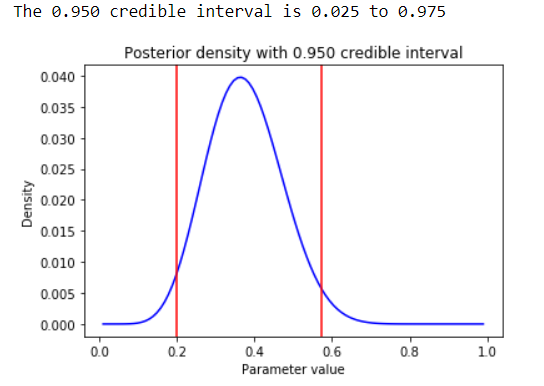
Because the posterior distribution above is symmetric, similar the beta prior we chose, the analysis is identical to CI'south in the frequentist approach. We tin can be 95% confident that around 40% of commuter's tested at this intersection during a red light will take COVID-nineteen! This info is very useful for wellness agencies to allocate resource appropriately.
If y'all remember the joke in the tertiary paragraph, about the Bayesian who vaguely suspected a horse and caught a fleeting glimpse of a donkey and strongly suspects seeing a mule — I hope you can now assign each clause of the joke the appropriate role Bayes theorem.
Check out my next piece on linear regression and using bootstrap with regression models.
Notice me on Linkedin
Physicist cum Data Scientist- Available for new opportunity | SaaS | Sports | Start-ups | Scale-ups
Source: https://towardsdatascience.com/bayesian-statistics-11f225174d5a
0 Response to "Is This Bayesian? You Know Im a Strict Bayesian"
Postar um comentário